
General purpose, courtesy of Python NLTK:
Movie review data, courtesy of the Large Movie Review Dataset. Provides 25,000 for training and 25,000 for testing:
General purpose, courtesy of Python NLTK:
Movie review data, courtesy of the Large Movie Review Dataset. Provides 25,000 for training and 25,000 for testing:
A quick Google search rendered two respectable solutions:
EXIF is a metdata specification largely used by modern versions of JPEG and TIFF. It allows you embed a wealth of descriptive information into a picture taken by your camera. Notably, this also, usually, includes one or more timestamps. In the event that you find yourself with a directory of anonymously-named images that you’d like to rename with their timestamps, I’ve written a quick Python script to automate such a task. This script assumes that you have the exif tool installed. It’s readily available for both Linux and Mac OS.
import os
import subprocess
import glob
import datetime

_PICTURE_PATH = '/my/pictures/are/here'

_EXIF_COMMAND = 'exif'
_FILESPEC = '*.jpg'
_NEW_FILENAME_TEMPLATE = '{timestamp_phrase}.jpg'
_COMMON_EXIF_TIMESTAMP_FIELD_NAME = 'Date and Time'
_EXIF_TIMESTAMP_FORMAT = '%Y:%m:%d %H:%M:%S'
_OUTPUT_TIMESTAMP_FORMAT = '%Y%m%d-%H%M%S'

def _get_exif_info(filepath):
    cmd = [_EXIF_COMMAND, '-m', filepath]
    p = subprocess.Popen(cmd, stdout=subprocess.PIPE)
    exif_tab_delimited = p.stdout.read()
    r = p.wait()
    if r != 0:
        raise ValueError("EXIF command failed: %s" % (cmd,))

    lines = exif_tab_delimited.strip().split('n')[1:]
    pairs = [l.split('t') for l in lines]
    return dict(pairs)

def _get_filepaths(path):
    full_pattern = os.path.join(path, _FILESPEC)
    for filepath in glob.glob(full_pattern):
        yield filepath

def _main():
    for original_filepath in _get_filepaths(_PICTURE_PATH):
        exif = _get_exif_info(original_filepath)

        try:
            exif_timestamp_phrase = exif[_COMMON_EXIF_TIMESTAMP_FIELD_NAME]
        except KeyError:
            print("ERROR: {0}: Missing timestamp field".format(original_filepath))
            print('')

            continue

        timestamp_dt =
            datetime.datetime.strptime(
                exif_timestamp_phrase,
                _EXIF_TIMESTAMP_FORMAT)

        output_timestamp_phrase =
            timestamp_dt.strftime(_OUTPUT_TIMESTAMP_FORMAT)

        new_filename = _NEW_FILENAME_TEMPLATE.format(
                        timestamp_phrase=output_timestamp_phrase)

        new_filepath = os.path.join(path, new_filename)

        print("{0} => {1}".format(original_filepath, new_filepath))
        os.rename(original_filepath, new_filepath)

if __name__ == '__main__':
    _main()
_PICTURE_PATH to the path of your pictures._FILESPEC to the correct pattern/casing of your files._COMMON_EXIF_TIMESTAMP_FIELD_NAME to the correct EXIF field-name if the device that created the pictures used a different field-name (you can use the exif tool directly to explore your images)._EXIF_TIMESTAMP_FORMAT to reflect the proper format.$ python rename_images.py
Success output will look something like:
./IMG_3871.jpg => ./20131127-143832.jpg
./IMG_3872.jpg => ./20131127-143836.jpg
./IMG_3879.jpg => ./20131127-144045.jpg
./IMG_3880.jpg => ./20131127-144105.jpg
./IMG_3927.jpg => ./20131128-172021.jpg
...
This is an example of how to use the boto library in Python to perform large, multipart, concurrent uploads to Amazon Glacier.
#!/usr/bin/env python2.7

import os.path

import boto.glacier.layer2

def upload(access_key, secret_key, vault_name, filepath, description):
l = boto.glacier.layer2.Layer2(
aws_access_key_id=access_key,
aws_secret_access_key=secret_key)

v = l.get_vault(vault_name)

archive_id = v.concurrent_create_archive_from_file(
filepath,
description)

print(archive_id)

if __name__ == '__main__':
access_key = 'XXX'
secret_key = 'YYY'
vault_name = 'images'
filepath = '/mnt/array/backups/big_archive.xz'
description = os.path.basename(filepath)

upload(access_key, secret_key, vault_name, filepath, description)
Amazon Glacier is a backup service that trades cost for convenience. It’s built around the concept of archive-files: Upload a single archive to your vault immediately, request the download of an archive from a vault and wait for four-hours for it to be fulfilled, or request an inventory of what you currently have stored in a particular vault (which also takes four-hours to fulfill). You can provide an Amazon Simple Notification Service resource in order to get an email or other type of notification when your inventory or download is ready.
Before proceeding, it’s worth mentioning the advantages of uploading several large archives rather than many small ones:
We’re using a tool called glacier_tool to perform the upload. This is a tool to perform fast, multipart, concurrent uploads. It was written because the author had an issue finding anything that already existed and was still maintained. Most of what other tools were found were either UI-based or didn’t seem to support multipart uploads.
The backend Amazon library currently has issues. One of them is buggy Python 3 support. So, make sure you have Python 2.7 and install via PyPI:
$ sudo pip install glacier_tool
$ export AWS_ACCESS_KEY=XXX
$ export AWS_SECRET_KEY=YYY

$ gt_upload_large -em 11.33 image-backups /mnt/tower/backups/images-main-2010-20150617-2211.tar.xz images-main-2010-20150617-2211.tar.xz
Uploading: [/mnt/array/backups/images-main-2010-20150617-2211.tar.xz]
Size: (15.78) G
Start time: [2015-07-05 01:22:01]
Estimated duration: (3.17) hours => [2015-07-05 04:32:11] @ (11.33) Mbps
Archive ID: [IEGZ8uXToCDIgO3pMrrIHBIcJs...YyNlPigEwIR2NA]
Duration: (3.16) hours @ (11.37) Mbps

$ gt_upload_large -em 11.37 image-backups /mnt/tower/backups/images-main-2011-20150617-2211.tar.xz images-main-2011-20150617-2211.tar.xz
Uploading: [/mnt/array/backups/images-main-2011-20150617-2211.tar.xz]
Size: (26.66) G
Start time: [2015-07-05 10:07:58]
Estimated duration: (5.33) hours => [2015-07-05 15:28:03] @ (11.37) Mbps
Note that the output of one upload will print the approximate rate at which the upload was performed. This can be fed into subsequent commands to estimate how long they will take to complete.
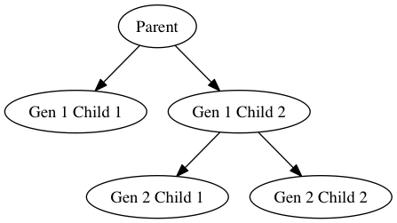
We’ll use the graphviz library to generate DOT-formatted data, and the dot command to generate an image:
import subprocess

import graphviz

_RENDER_CMD = ['dot']
_FORMAT = 'png'

def build():
    comment = "Test comment"
    dot = graphviz.Digraph(comment=comment)

    dot.node('P', label='Parent')
    dot.node('G1C1', label='Gen 1 Child 1')
    dot.node('G1C2', label='Gen 1 Child 2')
    dot.node('G2C1', label='Gen 2 Child 1')
    dot.node('G2C2', label='Gen 2 Child 2')

    dot.edge('P', 'G1C1')
    dot.edge('P', 'G1C2')
    dot.edge('G1C2', 'G2C1')
    dot.edge('G1C2', 'G2C2')

    return dot

def get_image_data(dot):
    cmd = _RENDER_CMD + ['-T' + _FORMAT]
    p = subprocess.Popen(
            cmd,
            stdin=subprocess.PIPE,
            stdout=subprocess.PIPE,
            stderr=subprocess.PIPE)

    (stdout, stderr) = p.communicate(input=dot)
    r = p.wait()

    if r != 0:
        raise ValueError("Command failed (%d):n"
                         "Standard output:n%sn"
                         "Standard error:n%s" %
                         (r, stdout, stderr))

    return stdout

dot = build()
dot_data = get_image_data(dot.source)

with open('output.png', 'wb') as f:
    f.write(dot_data)
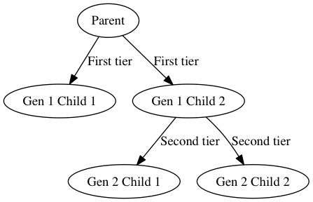
Note that we can provide labels for the edges, too. However, they tend to crowd the actual edges and it has turned out to be non-trivial to add margins to them:
Note that there are other render commands available for different requirements. This list is from the homepage:
This is an example of sfdp with the “-Goverlap=scale” argument with a very large graph (zoomed out).

If you’re running OS X, I had to uninstall graphviz, install the gts library, and then reinstall graphviz with an extra option to bind it:
$ brew uninstall graphviz
$ brew install gts
$ brew install --with-gts graphviz
If graphviz hasn’t been built with gts, you will get the following error:
Standard error:
Error: remove_overlap: Graphviz not built with triangulation library
Python provides regular-expression-based baked-in string-templating functionality. It’s highly configurable and allows you to easily do string-replacements into templates of the following manner:
Token 1: $Token1
Token 2: $Token2
Token 3: ${Token3}
You can tell it to use an alternate template pattern (using an alternate symbol or symbols) as well as being able to tell it to work differently at the regular-expression level.
It’s not spelled-out how to extract the tokens from a template, however. You would just use a simple regular-expression-based search:
import string
import re

text = """
Token 1: $Token1
Token 2: $Token2
Token 3: $Token3
"""

t = string.Template(text)
result = re.findall(t.pattern, t.template)
tokens = [r[1] for r in result]
print(tokens)
#['Token1', 'Token2', 'Token3']
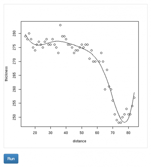
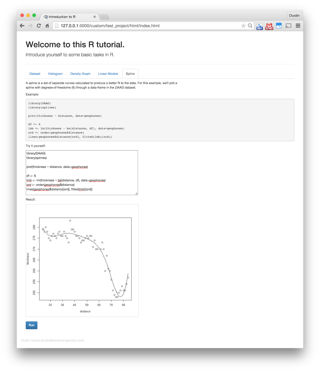
There is very limited coverage on how to build a website with R. It was a fight to answer the questions that I had. Obviously, this is because R was not meant to serve websites. In fact, if you want to serve a website that has any sort of volume, you’re probably better-off using Shiny Server or hosted Shinyapps.io: http://shiny.rstudio.com/deploy
However, you still may want to write your own R-based web application for one or more of the following reasons:
So, assuming that you just want to run your own server, I’ve created a test-project to help you out. Make sure to install the requirements before running it. The project depends on the DAAG package. This is a companion package to a book that we use for the dataset in a spline example.
This project was created on top of Rook, a fairly low-level R package that removes most of the semantics of serving web-requests while still leaving you buried in the flow. This was brought about by Jeffrey Horner who had previously introduced both rApache and Brew. He was also involved in Shiny Server’s implementation.
We’ll include a couple of excerpts from the project, here. For more information on running the example project, go to the project website.
The main routing code:
#!/usr/bin/env Rscript

library(Rook)

source('ajax.r')

main.app <- Builder$new(
    # Static assets (images, Javascript, CSS)
    Static$new(
        urls = c('/static'),
        root = '.'
    ),

    # Webpage serving.
    Static$new(urls='/html',root='.'),

    Rook::URLMap$new(
        '/ajax/lambda/result' = lambda.ajax.handler,
        '/ajax/lambda/image' = lambda.image.ajax.handler,
        '/' = Redirect$new('/html/index.html')
    )
)

s <- Rhttpd$new()
s$add(name='test_project',app=main.app)

s$start(port=5000)

while (TRUE) {
    Sys.sleep(0.5);
}
We loop at the bottom because, if you’re calling this as a script as intended, we want to keep it running in order to process requests.
The dynamic-request handlers:
library(jsonlite)
library(base64enc)

source('utility.r')

eval.code <- function(code, result_name=NULL) {
    message <- NULL
    cb_error <- function(e) {
        message <<- list(type='error', message=e$message)
    }
    cb_warning <- function(w) {
        message <<- list(type='warning', message=w$message)
    }

    tryCatch(eval(parse(text=code)), error=cb_error, warning=cb_warning)

    if(is.null(message)) {
        result <- list(success=TRUE)

        if(is.null(result_name) == FALSE) {
            if(exists(result_name) == FALSE) {
                result$found <- FALSE
            } else {
                result$found <- TRUE
                result$value <- mget(result_name)[[result_name]]
            }
        }

        return(result)
    } else {
        return(list(success=FALSE, message=message))
    }
}

lambda.ajax.handler <- function(env) {
    # Execute code and return the value for the variable of the given name.

    req <- Request$new(env)

    if(is.null(req$GET()$tab_name)) {
        # Parameters missing.
        res <- Response$new(status=500)
        write.text(res, "No 'tab_name' parameter provided.")
    } else if(is.null(req$GET()$result_name)) {
        # Parameters missing.
        res <- Response$new(status=500)
        write.text(res, "No 'result_name' parameter provided.")
    } else if(is.null(req$POST())) {
        # Body missing.
        res <- Response$new(status=500)
        write.text(res, "POST-data missing. Please provide code.")
    } else {
        # Execute code and return the result.

        res <- Response$new()

        result_name <- req$GET()$result_name
        code <- req$POST()[['code']]

        execution_result <- eval.code(code, result_name=result_name)
        execution_result$value = paste(capture.output(print(execution_result$value)), collapse='n')

        write.json(res, execution_result)
    }

    res$finish()
}

lambda.image.ajax.handler <- function(env) {
    # Execute code and return a base64-encoded image.

    req <- Request$new(env)

    if(is.null(req$GET()$tab_name)) {
        # Parameters missing.
        res <- Response$new(status=500)
        write.text(res, "No 'tab_name' parameter provided.")
    } else if(is.null(req$POST())) {
        # Body missing.
        res <- Response$new(status=500)
        write.text(res, "POST-data missing. Please provide code.")
    } else {
        # Execute code and return the result.

        # If we're returning an image, set the content-type and redirect
        # the graphics device to a file.

        t <- tempfile()
        png(file=t)
        png(t, type="cairo", width=500, height=500)

        result_name <- req$GET()$result_name
        code <- req$POST()[['code']]

        execution_result <- eval.code(code, result_name=result_name)

        # If we're returning an image, stop the graphics device and return
        # the data.

        dev.off()
        length <- file.info(t)$size

        if(length == 0) {
            res <- Response$new(status=500)
            res$header('Content-Type', 'text/plain')

            res$write("No image was generated. Your code is not complete.")
        } else {
            res <- Response$new()
            res$header('Content-Type', 'text/plain')

            data_uri <- dataURI(file=t, mime="image/png")
            res$write(data_uri)
        }
    }

    res$finish()
}
For reference, there is also another project called rapport that lets you produce HTML though not whole websites.

Of the five or six most well-known charting packages, none really impressed me (being a devoted user of Highcharts, in Javascript). The exception to this is plot.py but it’s a remote service and I’d rather not couple myself to a service.
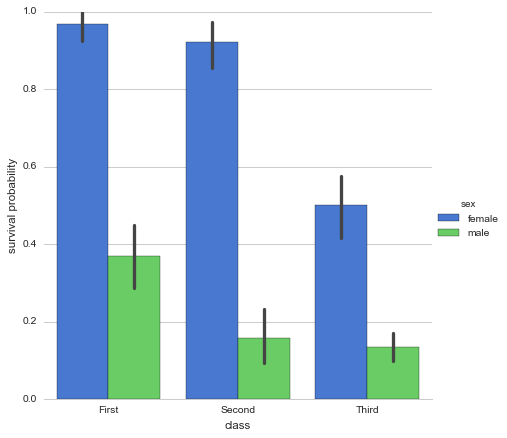
In the end, I went with Seaborn (Stanford). This seemed to look the best of all of the options, even if it was tough to get some of the features working right. They recently added a chart for the exclusive purpose of plotting categorical/factor-based data: factorplot.
An example of Seaborn’s factorplot:
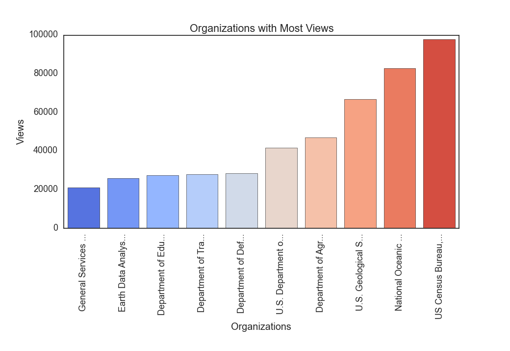
I put together an example of a bar-chart using data from data.gov. I used pandas to read the CSV data. Since Seaborn is built on top of matplotlib and matplotlib appears to have issues displaying graphics in my local environment, I had to rely on running the example via ipython using the matplotlib magic function (which loads everything necessary and worked as expected).
To run the example, you’ll need the following packages (in addition to the ipython environment):
The code:
# Tell ipython to load the matplotlib environment.
%matplotlib

import itertools

import pandas
import numpy
import seaborn
import matplotlib.pyplot

_DATA_FILEPATH = 'datagovdatasetsviewmetrics.csv'
_ROTATION_DEGREES = 90
_BOTTOM_MARGIN = 0.35
_COLOR_THEME = 'coolwarm'
_LABEL_X = 'Organizations'
_LABEL_Y = 'Views'
_TITLE = 'Organizations with Most Views'
_ORGANIZATION_COUNT = 10
_MAX_LABEL_LENGTH = 20

def get_data():
    # Read the dataset.

    d = pandas.read_csv(_DATA_FILEPATH)

    # Group by organization.

    def sum_views(df):
        return sum(df['Views per Month'])

    g = d.groupby('Organization Name').apply(sum_views)

    # Sort by views (descendingly).

    g.sort(ascending=False)

    # Grab the first N to plot.

    items = g.iteritems()
    s = itertools.islice(items, 0, _ORGANIZATION_COUNT)

    s = list(s)

    # Sort them in ascending order, this time, so that the larger ones are on
    # the right (in red) in the chart. This has a side-effect of flattening the
    # generator while we're at it.
    s = sorted(s, key=lambda (n, v): v)

    # Truncate the names (otherwise they're unwieldy).

    distilled = []
    for (name, views) in s:
        if len(name) > (_MAX_LABEL_LENGTH - 3):
            name = name[:17] + '...'

        distilled.append((name, views))

    return distilled

def plot_chart(distilled):
    # Split the series into separate vectors of labels and values.

    labels_raw = []
    values_raw = []
    for (name, views) in distilled:
        labels_raw.append(name)
        values_raw.append(views)

    labels = numpy.array(labels_raw)
    values = numpy.array(values_raw)

    # Create one plot.

    seaborn.set(style="white", context="talk")

    (f, ax) = matplotlib.pyplot.subplots(1)

    b = seaborn.barplot(
        labels,
        values,
        ci=None,
        palette=_COLOR_THEME,
        hline=0,
        ax=ax,
        x_order=labels)

    # Set labels.

    ax.set_title(_TITLE)
    ax.set_xlabel(_LABEL_X)
    ax.set_ylabel(_LABEL_Y)

    # Rotate the x-labels (otherwise they'll overlap). Seaborn also doesn't do
    # very well with diagonal labels so we'll go vertical.
    b.set_xticklabels(labels, rotation=_ROTATION_DEGREES)

    # Add some margin to the bottom so the labels aren't cut-off.
    matplotlib.pyplot.subplots_adjust(bottom=_BOTTOM_MARGIN)

distilled = get_data()
plot_chart(distilled)
To run the example, save it to a file and load it into the ipython environment. If you were to save it as “barchart.ipy” (using the “ipy” extension so it processes the %matplotlib directive properly) and then start ipython using the “ipython” executable, you’d load it like this:
%run barchart.ipy
The graphic will be displayed in another window:
I should also mention that I really like pygal but didn’t consider it an option because I wanted a traditional, flat image, not an SVG. Even so, here’s an example from their website:
import pygal                                                       # First import pygal
bar_chart = pygal.Bar()                                            # Then create a bar graph object
bar_chart.add('Fibonacci', [0, 1, 1, 2, 3, 5, 8, 13, 21, 34, 55])  # Add some values
bar_chart.render_to_file('bar_chart.svg')                          # Save the svg to a file
Output:
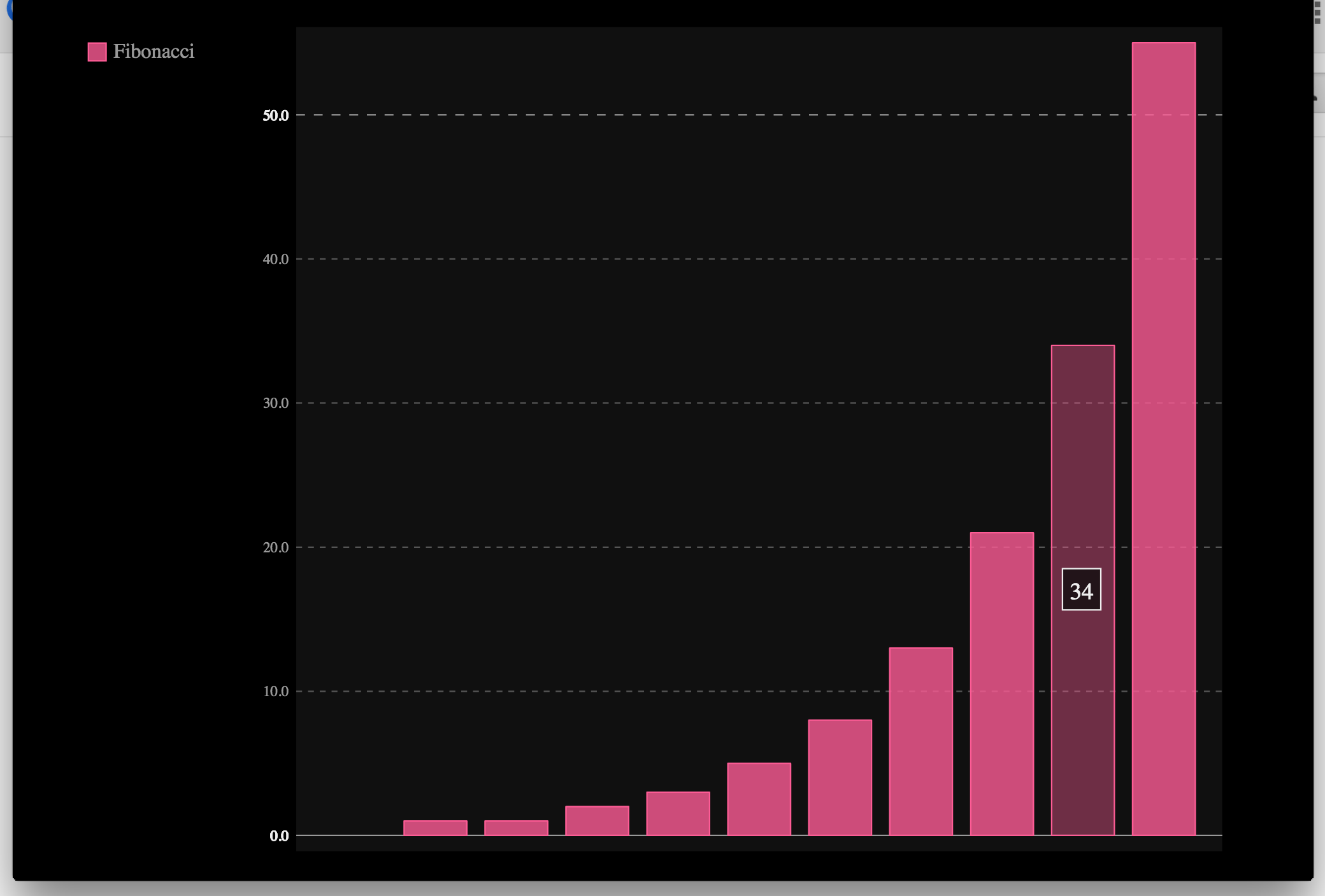
Notice that the resulting SVG even has hover effects.
I just noticed a Superuser question with ~80000 views where people were still generally-clueless about a commandline trick with file-copying. As there was only a slight variation of this mentioned, I’m going to share it here.
So, the following command can be interpreted two different ways:
$ cp -r dir1 dir2
dir2 exists, copy dir1 into dir2 as basename(dir1).dir2 doesn’t exist, copy dir1 into dirname(dir2) and name it basename(dir1).What if you want to always copy the contents of dir1 into dir2? Well, you’d do this:
$ cp -r dir1/* dir2
However, this will ignore any hidden files in dir1. Instead, you can add a trailing slash to dir1:
$ cp -r dir1/ dir2
This will deterministically pour the contents of dir1 into dir2.
Example:
/tmp$ mkdir test_dir1
/tmp$ cd test_dir1/
/tmp/test_dir1$ touch aa
/tmp/test_dir1$ touch .bb
/tmp/test_dir1$ cd ..
/tmp$ mkdir test_dir2

/tmp$ cp -r test_dir1/* test_dir2
/tmp$ ls -1a test_dir2
.
..
aa

/tmp$ cp -r test_dir1/ test_dir2
/tmp$ ls -1a test_dir2
.
..
.bb
aa
The Superuser question insisted that you needed a period at the end of the from argument which isn’t accurate (but will still work).

You must be logged in to post a comment.